rpact: An R Package For Adaptive Clinical Trials

ROeS 2025, Graz

Gernot Wassmer, Friedrich Pahlke, Daniel Sabanés Bové

RPACT GbR

September 16, 2025

Overview 📦

• Comprehensive validated R package implementing methodology described in Wassmer and Brannath (2016)
• Enables the design of traditional and confirmatory adaptive group sequential designs
• Provides interim data analysis and simulation including early efficacy stopping and futility analyses
• Enables sample-size reassessment with different strategies
• Enables treatment arm selection in multi-stage multi-arm (MAMS) designs
• Enables subset selection in population enrichment designs
• Provides a comprehensive and reliable sample size calculator

Developed by RPACT 🏢

• RPACT company founded in 2017 by Gernot Wassmer and Friedrich Pahlke
• Idea: open source development with help of “crowd funding”
• Currently supported by 21 companies
• \(>\) 80 presentations and training courses since 2018, e.g., FDA in March 2022
• 29 vignettes based on Quarto and published on rpact.org/vignettes
• 28 releases on CRAN since 2018

RCONIS 🚀

• Grow RPACT company to offer a wider range of services
• Statistical consulting and engineering services: Research Consulting and Innovative Solutions
• Joint venture between RPACT GbR (rpact.com) and inferential.biostatistics GmbH (inferential.bio) founded by Daniel Sabanés Bové and Carrie Li
• Website: rconis.com

The R Package rpact – Functional Range

Trial Designs 🔬

• Fixed sample designs:
  • continuous, binary, count, survival outcomes
• Group sequential designs:
  • efficacy interim analyses, futility stopping, alpha-spending functions
• Adaptive designs:
  • Inverse normal and Fisher’s combination test, conditional error rate principle
  • Provides adjusted confidence intervals and bias corrected estimates
  • Multi-arm multi-stage (MAMS) and enrichment designs, sample size reassessment

Easy to understand R commands:

getDesignGroupSequential()
getDesignInverseNormal()
getDesignFisher()
getDesignConditionalDunnett()

Sample Size and Power Calculation 💻

Sample size and power can be calulcated for testing:

• means (continuous endpoint)
• proportions (binary endpoint)
• hazards (survival endpoint)
  • Note: flexible recruitment and survival time options
• rates (count endpoint)

Easy to understand R commands:

getSampleSize[Means / Rates / Survival / Counts]()
getPower[Means / Rates / Survival / Counts]()

Example: Sample Size Calculation 🧮

# Define the design.
getDesignGroupSequential(
    typeOfDesign = "asOF",
    futilityBounds = c(0, 0)
) |>
    # Perform sample size calculation.
    getSampleSizeMeans(
        alternative = 2,
        stDev = 5
    ) |>
    # Obtain summary.
    summary()

Sample size calculation for a continuous endpoint

Sequential analysis with a maximum of 3 looks (group sequential design), one-sided overall significance level 2.5%, power 80%. The results were calculated for a two-sample t-test, H0: mu(1) - mu(2) = 0, H1: effect = 2, standard deviation = 5.

Stage	1	2	3
Planned information rate	33.3%	66.7%	100%
Cumulative alpha spent	0.0001	0.0060	0.0250
Stage levels (one-sided)	0.0001	0.0060	0.0231
Efficacy boundary (z-value scale)	3.710	2.511	1.993
Futility boundary (z-value scale)	0	0
Efficacy boundary (t)	4.690	2.152	1.384
Futility boundary (t)	0	0
Cumulative power	0.0204	0.4371	0.8000
Number of subjects	69.9	139.9	209.8
Expected number of subjects under H1			170.9
Overall exit probability (under H0)	0.5001	0.1309
Overall exit probability (under H1)	0.0684	0.4202
Exit probability for efficacy (under H0)	0.0001	0.0059
Exit probability for efficacy (under H1)	0.0204	0.4167
Exit probability for futility (under H0)	0.5000	0.1250
Exit probability for futility (under H1)	0.0480	0.0035

Legend:

• (t): treatment effect scale

Adaptive Analysis 📈

• Perform interim and final analyses during the trial using group sequential method or p-value combination test (inverse normal or Fisher)

• Calculate adjusted point estimates and confidence intervals (cf., Robertson et al. (2023), Robertson et al. (2025))

• Perform sample size reassessment based on the observed data, based on calculation of conditional power

• Some highlights:

  • Automatic boundary recalculations during the trial for analysis with alpha spending approach, including under- and over-running
  • Adaptive analysis tools for multi-arm trials and enrichment designs

Easy to understand R commands:

getStageResults()
getRepeatedConfidenceIntervals()
getAnalysisResults()

Simulation Tool 🧪

Obtain operating characteristics of different designs:

• Assessment of adaptive sample size recalculation strategies
• Assessment of treatment selection strategies in multi-arm trials
• Assessment of population selection strategies in enrichment designs

Easy to understand R commands:

getSimulation[MultiArm / Enrichment][Means / Rates / Survival / Counts]()

Example:

getSimulationMeans()
getSimulationMultiArmMeans()
getSimulationEnrichmentMeans()

Recent Updates

1. Count Data

• getSampleSizeCounts() and getPowerCounts()
  • Perform sample size calculations and the assessment of test characteristics for clinical trials with negative binomial distributed count data.
  • Fixed sample size and group sequential designs (Mütze et al. (2019))
  • Perform blinded sample size reassessments according to Friede and Schmidli (2010)
  • Output boundary values also on the treatment effect scale
• New function getSimulationCounts()
  • Perform power simulations for clinical trials with negative binomial distributed count data
  • Simulated power, stopping probabilities, conditional power, and expected sample size for testing mean rates for negative binomial distributed event numbers in the two treatment groups testing situation

Count Data: Options

• Either both event rates \(\lambda_1\) and \(\lambda_2\), or \(\lambda_2\) and rate ratio \(\theta\), or \(\lambda\) and \(\theta\) (blinded sample size reassessment!)
• \(\lambda_1\) and \(\theta\) can be vectors
• Different ways of calculation:
  • fixed exposure time,
  • accrual and study time,
  • or accrual and fixed number of patients
• Staggered patient entry
• Group sequential or fixed sample size setting

Count Data: Simple Example

getSampleSizeCounts(
    alpha = 0.05,
    beta = 0.1,
    sided = 2,
    lambda2 = 0.4,
    theta = 0.75,
    overdispersion = 0.5,
    fixedExposureTime = 1
) |> summary()

Count Data: Simple Example

Sample size calculation for a count data endpoint

Fixed sample analysis, two-sided significance level 5%, power 90%. The results were calculated for a two-sample Wald-test for count data, H0: lambda(1) / lambda(2) = 1, H1: effect = 0.75, lambda(2) = 0.4, overdispersion = 0.5, fixed exposure time = 1.

Stage	Fixed
Stage level (two-sided)	0.0500
Efficacy boundary (z-value scale)	1.960
Lower efficacy boundary (t)	0.844
Upper efficacy boundary (t)	1.171
Lambda(1)	0.300
Number of subjects	1736.0
Maximum information	127.0

Legend:

• (t): treatment effect scale

Count Data: Power Calculation

getPowerCounts(
    directionUpper = FALSE,
    lambda2 = 1.4,
    theta = c(0.75, 1),
    overdispersion = 0.7,
    maxNumberOfSubjects = 300,
    followUpTime = 12,
    accrualTime = 12
) |> fetch(overallReject)

$overallReject
[1] 0.8213803 0.0250000

Count Data: Power Simulation

tictoc::tic()
getSimulationCounts(
    directionUpper = FALSE,
    lambda2 = 1.4,
    theta = c(0.75, 1),
    overdispersion = 0.7,
    maxNumberOfSubjects = 300,
    plannedCalendarTime = 24,
    accrualTime = 12,
    fixedExposureTime = 12,
    # followUpTime = 12,
    maxNumberOfIterations = 1000,
    seed = 123
) |> fetch(overallReject)

$overallReject
[1] 0.835 0.028

tictoc::toc()

1.65 sec elapsed

2. Delayed Response

• The delayed response group sequential methodology from Hampson and Jennison (2013) defines a proper consideration of the “pipeline” patients who have been treated at interim but are yet to respond
• getDesignGroupSequential(), getDesignCharacteristics(), and the corresponding getSampleSizexxx() and getPowerxxx() functions characterize a delayed response group sequential test given certain input parameters in terms of power, maximum sample size and expected sample size
• Other approaches can conveniently be handled with the newly published function getGroupSequentialProbabilities()
• Details and examples provided in Vignette Delayed Response Design with rpact.

Methodology of Delayed Response Designs

Given boundary sets \(\{u^0_1,\dots,u^0_{K-1}\}\), \(\{u_1,\dots,u_K\}\) and \(\{c_1,\dots,c_K\}\), a \(K\)-stage delayed response group sequential design has the following structure:

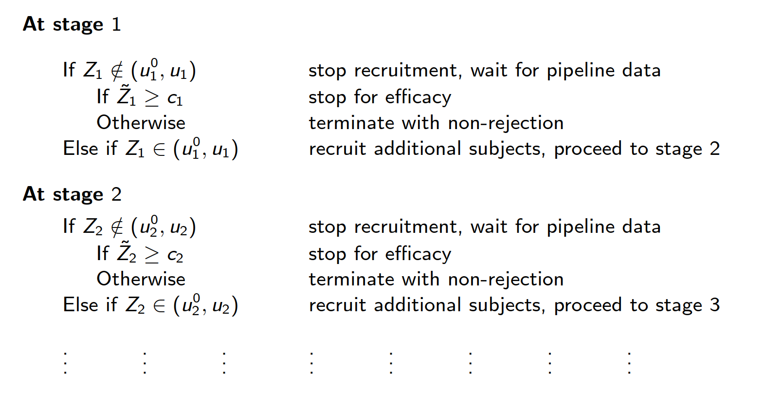
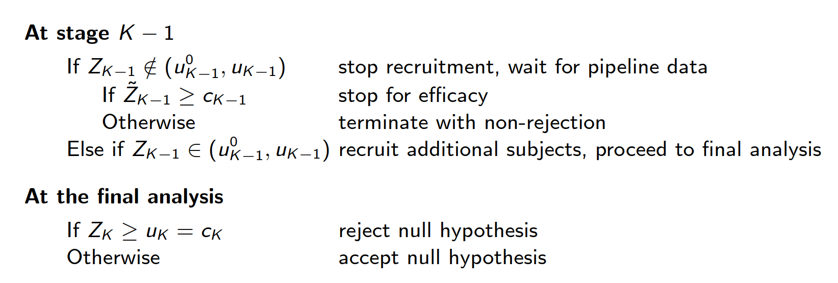
According to Hampson and Jennison (2013), the boundaries \(\{c_1, \dots, c_K\}\) with \(c_K = u_K\) are chosen such that “reversal probabilities” are balanced, to ensure type I error control.

More precisely, \(c_1,\ldots,c_{K - 1}\) are chosen as the (unique) solution of: \[\begin{align*} \begin{split} &P_{H_0}(Z_1 \in (u^0_1, u_1), \dots, Z_{k-1} \in (u^0_{k-1}, u_{k-1}), Z_k \geq u_k, \tilde{Z}_k \leq c_k) \\ &= P_{H_0}(Z_1 \in (u^0_1, u_1), \dots, Z_{k-1} \in (u^0_{k-1}, u_{k-1}), Z_k \leq u^0_k, \tilde{Z}_k \geq c_k). \end{split} \end{align*}\]

Delayed Response: Example

gsdWithDelay <- getDesignGroupSequential(
    kMax = 3,
    alpha = 0.025,
    beta = 0.2,
    typeOfDesign = "asKD",
    gammaA = 2,
    gammaB = 2,
    typeBetaSpending = "bsKD",
    informationRates = c(0.3, 0.7, 1),
    delayedInformation = c(0.16, 0.2),
    bindingFutility = TRUE
)
gsdWithDelay |> summary()

Delayed Response: Example

Sequential analysis with a maximum of 3 looks (delayed response group sequential design)

Kim & DeMets alpha spending design with delayed response (gammaA = 2) and Kim & DeMets beta spending (gammaB = 2), one-sided overall significance level 2.5%, power 80%, undefined endpoint, inflation factor 1.0514, ASN H1 0.9269, ASN H01 0.9329, ASN H0 0.8165.

Stage	1	2	3
Planned information rate	30%	70%	100%
Delayed information	16%	20%
Cumulative alpha spent	0.0022	0.0122	0.0250
Cumulative beta spent	0.0180	0.0980	0.2000
Stage levels (one-sided)	0.0022	0.0109	0.0212
Upper bounds of continuation	2.841	2.295	2.030
Lower bounds of continuation (binding)	-0.508	1.096
Decision critical values	1.387	1.820	2.030
Reversal probabilities	<0.0001	0.0018
Cumulative power	0.1026	0.5563	0.8000
Futility probabilities under H1	0.019	0.083

Delayed Response: Plot

gsdWithDelay |> plot()

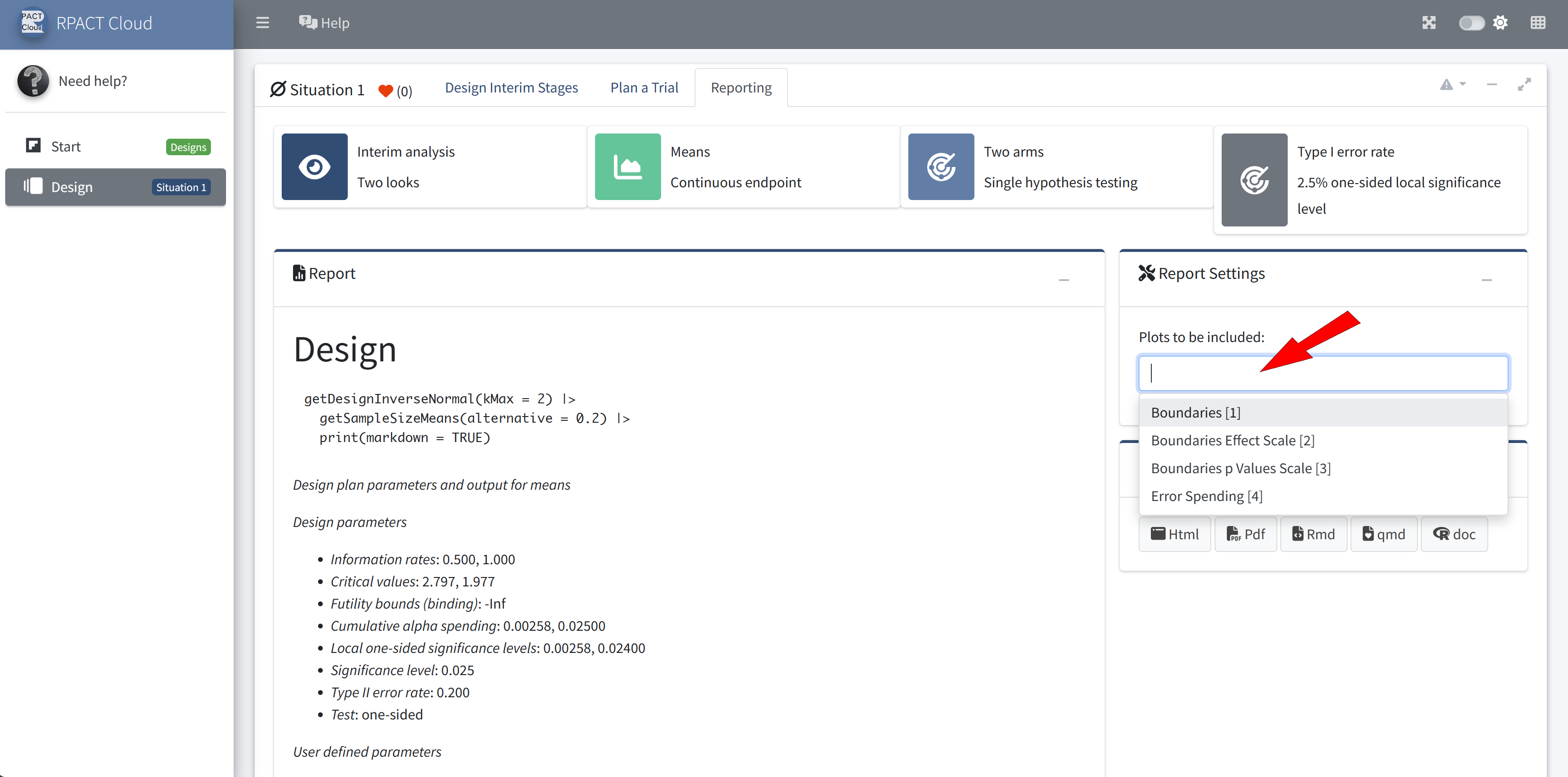
3. Conditional Performance Score

• Performance scores combine different performance criteria in one value (e.g. Liu, Zhu, and Cui (2008), Wu and Cui (2012))

• Evaluation perspectives: global and conditional

  • global: looking at the properties of the adaptive design before the study starts
  • conditional: looking at the properties of the adaptive design when the interim result suggests a trial continuation

Conditional Performance Score (cont’d)

• Idea of the conditional performance score:
  • Evaluation of second stage sample size update
  • Conditional power and sample size are random variables and therefore best described by location and variation measures
  • Score by Herrmann et al. (2020) consists of four components (location and variation of conditional power and sample size)
  • Score and its components take values between 0 and 1 (the higher the values, the better the performance)
  • Usage of getPerformanceScore() of a simulation object.

Conditional Performance Score: Example

# Initialize group sequential design with O'Brien-Fleming-boundaries
design <- getDesignGroupSequential(
    kMax = 2,
    typeOfDesign = "OF",
    futilityBounds = 0,
    bindingFutility = TRUE
)
# Perform simulation
maxNumberOfSubjects <- 200
n1 <- maxNumberOfSubjects * design$informationRates[1]
alternative <- c(0.2, 0.3, 0.4, 0.5)
design |>
    getSimulationMeans(
        alternative = alternative,
        plannedSubjects = c(n1, maxNumberOfSubjects),
        minNumberOfSubjectsPerStage = c(NA, 1),
        maxNumberOfSubjectsPerStage = c(NA, 2*maxNumberOfSubjects),
        conditionalPower = 0.8,
        maxNumberOfIterations = 1e05,
        seed = 123
    ) |>
    # Calculate performance score
    getPerformanceScore()

Conditional Performance Score: Example

Performance

• Location sample sizes: 0.3042, 0.9516, 0.7936, 0.7353
• Variation sample sizes: 0.2591, 0.2138, 0.2318, 0.3094
• Sub-score sample sizes: 0.2817, 0.5827, 0.5127, 0.5223
• Location conditional power: 0.7254, 0.8150, 0.8897, 0.9402
• Variation conditional power: 0.3691, 0.4391, 0.5460, 0.6560
• Sub-score conditional power: 0.5472, 0.6271, 0.7178, 0.7981
• Performance scores: 0.4144, 0.6049, 0.6153, 0.6602

RPACT Cloud

RPACT Cloud ☁️

• Graphical user interface

• Web based usage without local installation on nearly any device

• Provides an easy entry to to learn and demonstrate the usage of rpact

• Starting point for your R Markdown or Quarto reports

• Online available at cloud.rpact.com

Start Page

Design

Reporting

What’s Next?

New Package Features

Just in the near future you will see in rpact:

• Patient level survival data simulations for multi-arm and enrichment designs
• Optimum conditional error functions according to Brannath et al. (2024) (package optconerrf published on CRAN Sep 09, 2025)
• Least square means interface for continuous endpoints
• Additional futility boundary scales: function getFutilityBounds()
  • Available scales: zValue, pValue, conditionalPower, condPowerAtObserved, predictivePower, reverseCondPower, effectEstimate

Second Edition of the Book

• Provides up-to-date overview of group sequential and confirmatory adaptive designs in clinical trials
• Describes available software including R packages and has rpact code examples
• Supplemented with a discussion of practical applications

The R Package rpact - Online Resources

Further information, installation, and usage:

• CRAN: cran.r-project.org/package=rpact
• GitHub: github.com/rpact-com/rpact
• GitHub Pages: rpact-com.github.io/rpact
• OpenSci R-universe: rpact-com.r-universe.dev/rpact
• METACRAN: r-pkg.org/pkg/rpact
• Codecov: app.codecov.io/gh/rpact-com/rpact
• RPACT manual and vignettes: rpact.org
• RPACT validation and training: rpact.com

All information and resources about RPACT on one dashboard page

RPACT Connect: connect.rpact.com

RPACT Connect

Thank you!

References

Brannath, W., M. Dreher, J. Verth, and M. Scharpenberg. 2024. “Optimal Monotone Conditional Error Functions.” arXiv Preprint arXiv:2402.00814.

Friede, Tim, and Heinz Schmidli. 2010. “Blinded Sample Size Reestimation with Count Data: Methods and Applications in Multiple Sclerosis.” Statistics in Medicine 29 (10): 1145–56. https://doi.org/https://doi.org/10.1002/sim.3861.

Hampson, Lisa V., and Christopher Jennison. 2013. “Group Sequential Tests for Delayed Responses (with Discussion).” Journal of the Royal Statistical Society Series B: Statistical Methodology 75 (1): 3–54. https://doi.org/10.1111/j.1467-9868.2012.01030.x.

Herrmann, Carolin, Maximilian Pilz, Meinhard Kieser, and Geraldine Rauch. 2020. “A New Conditional Performance Score for the Evaluation of Adaptive Group Sequential Designs with Sample Size Recalculation.” Statistics in Medicine 39 (15): 2067–2100. https://doi.org/https://doi.org/10.1002/sim.8534.

Liu, G. Frank, G. Ray Zhu, and Lu Cui. 2008. “Evaluating the Adaptive Performance of Flexible Sample Size Designs with Treatment Difference in an Interval.” Statistics in Medicine 27 (4): 584–96. https://doi.org/https://doi.org/10.1002/sim.2998.

Mütze, Tobias, Ekkehard Glimm, Heinz Schmidli, and Tim Friede. 2019. “Group Sequential Designs for Negative Binomial Outcomes.” Statistical Methods in Medical Research 28 (8): 2326–47. https://doi.org/10.1177/0962280218773115.

Robertson, David S, Thomas Burnett, Babak Choodari-Oskooei, Munya Dimairo, Michael Grayling, Philip Pallmann, and Thomas Jaki. 2025. “Confidence Intervals for Adaptive Trial Designs I: A Methodological Review.” Statistics in Medicine 44 (18-19): e70174.

Robertson, David S, Babak Choodari-Oskooei, Munya Dimairo, Laura Flight, Philip Pallmann, and Thomas Jaki. 2023. “Point Estimation for Adaptive Trial Designs i: A Methodological Review.” Statistics in Medicine 42 (2): 122–45.

Wassmer, Gernot, and Werner Brannath. 2016. Group Sequential and Confirmatory Adaptive Designs in Clinical Trials. Springer. https://link.springer.com/book/10.1007/978-3-319-32562-0.

Wu, Xiaoru, and Lu Cui. 2012. “Group Sequential and Discretized Sample Size Re-Estimation Designs: A Comparison of Flexibility.” Statistics in Medicine 31 (24): 2844–57. https://doi.org/https://doi.org/10.1002/sim.5395.